Please note: We get commissions for purchases made through links in this post. This is to help support our blog and does not have impact on our recommendations. See disclosure for details.
The following figure shows an interactive oscilloscope simulator for the internet browser (requires Javascript). The black controls (Time/div, Volt/div, etc.) can be adjusted with the mouse or with the finger and are clickable. Repeated clicking rotates the buttons or switches until they return to their original position.
Short Instruction for the Oscilloscope Simulator
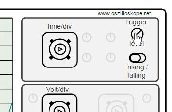
Oscilloscope simulator: The cursor changes to a hand over the switchable controls (Chrome-Browser).
The upper part of the simulator shows the oscilloscope, the lower part a frequency generator directly connected to the oscilloscope. Only one channel is used. The oscilloscope layout is divided into the parts display, time base and level setting (see oscilloscope usage). The area "trigger" shows the trigger level as well as the rising/fall gradient. Also the slope can be selected (=increasing/decreasing). The trigger is triggered when the signal reaches the trigger level and the edge rises accordingly, depending on the setting. The trigger level is defined by a green bar in the display of the oscilloscope and scales with the voltage range. The representation shows the signal amplitude per div and the time base setting in the upper part of the display.
The frequency generator has two setting options. The rotary switch "Amplitude" selects the peak-to-peak amplitude of the sine wave. A setting of e.g. 20 mV means that the sine wave oscillates from 0 to 20mV. The rotary switch "Frequency" sets the frequency of the sine wave. Both values are shown in the display of the frequency generator.
Examples

Oscilloscope simulator: The signal is in saturation and is cut off at the top of the display.
A setting as shown in the above illustration leads to a saturation of the signals. The oscillation amplitude of 10mV exceeds the display range at a volt/div setting of 1mV. The display height is eight boxes, i.e. at given setting it can only measure up to 8mV.

Oscilloscope simulator: Trigger level is greater than the signal amplitude or the slope does not trigger (here: Trigger level=10 mV, but rising trigger is not triggered, since the sine signal drops again after the maximum level of 10mV).
A setting like on this screen does not trigger the scope. Here the trigger level is 10mV, the slope is set to "Rising". At 10mV you can only "catch" the maxima of the sinusoidal oscillation that occurs immediately after the apex but falls off. In such a case you have to either switch the slope or decrease the trigger level.

Oscilloscope simulator: Artifacts occur at high frequencies due to discrete sampling. The signal is sampled internally in the simulator at approx. 100kHz.
This setting symbolizes an effect that is often seen while sampling high-frequency signals. Here, the sampling rate and the signal frequency are too close to each other. The signal frequency is 50kHz. The internal sampling rate of the oscilloscope is 105.5kHz (to avoid unnecessary simulation time on low-power smartphones), i.e. approx. a factor 2 above the signal frequency. The simulator uses a simple reconstruction of the sampled data. The data points are only connected by a line. A sampling near the cut-off frequency leads to a few sampling points per period and thus to a falsified representation of the signal. Through zeropadding and filtering the result can be improved. More information can be found in the article on the signal reconstruction.
We get commissions for purchases made through links in this post.